Outputs
By default, all outputs are written to a folder in local_results/ entitled folder_label_yyyy-mm-dd-hh:mm:ss
backend.h5
H5 file containing the entire chain from the MCMC and the corresponding log-likelihood values. This is updated continuously. If the code crashes, all existing results are still present. H5 files can be re-loaded as the current state for the MCMC at the beginning of another run (see the main method in blazar_run_mcmc.py) or loaded to use for statistics or plotting (see load_backend() in blazar_report.py).
Text files
basic_info.txt
Contains information from the configurations file, some paths and the running time. e.g.
folder name: local_results/J1010_2023-07-04-23:03:45
report description: J1010

config file: mcmc_config.txt
prev_files: False, use_param_file: False

configurations:
{'description': 'J1010', 'folder_label': 'J1010', 'eic': False, 'data_file': 'real_data/J1010_SED_reduced.dat', 'n_steps': 5000, 'n_walkers': 100, 'discard': 200, 'parallel': True, 'cores': 15, 'use_variability': True, 'tau_variability': 24.0, 'redshift': 0.143, 'custom_alpha2_limits': False, 'bb_temp': 'null', 'l_nuc': 'null', 'tau': 'null', 'blob_dist': 'null', 'alpha2_limits': [1.5, 7.5], 'fixed_params': [-inf, -inf, -inf, -inf, -inf, -inf, -inf, -inf, -inf]}

p0: random

time: 5:45:22.151980
info.txt
Main output containing the best fit parameters with associated errors, and statistical information. e.g.
configurations:
{'description': 'J1010_quicktest', 'folder_label': 'J1010', 'eic': False, 'data_file': 'real_data/J1010_SED_reduced.dat', 'n_steps': 100, 'n_walkers': 50, 'discard': 20, 'parallel': True, 'cores': 15, 'use_variability': True, 'tau_variability': 24.0, 'redshift': 0.143, 'custom_alpha2_limits': False, 'bb_temp': 'null', 'l_nuc': 'null', 'tau': 'null', 'blob_dist': 'null', 'alpha2_limits': [1.5, 7.5], 'fixed_params': [83.8, -inf, -inf, -inf, -inf, -inf, -inf, -inf, -inf]}

Parameter    Best Value       1sigma Range
    K         2.98e+04    2.98e+04 - 2.98e+04
 alpha_1      2.90e+00    2.90e+00 - 2.90e+00
 alpha_2      5.84e+00    5.84e+00 - 5.84e+00
gamma_min     5.29e+02    5.29e+02 - 5.29e+02
gamma_max     3.56e+06    3.56e+06 - 3.56e+06
gamma_break    2.09e+05    2.09e+05 - 2.09e+05
    B         2.08e-02    2.08e-02 - 2.08e-02
    R         5.05e+16    5.05e+16 - 5.05e+16
Reduced chi squared: 279.39 / 26 = 10.75


best params: [ 4.4744869   2.90451014  5.83862833  2.72311678  6.55186859  5.32035444
-1.68218932 16.70306255], chi squared = 279.38725352463666

min_1sigma_params: [ 4.4744869   2.90451014  5.83862833  2.72311678  6.55186859  5.32035444
-1.68218932 16.70306255]
max_1sigma_params: [ 4.4744869   2.90451014  5.83862833  2.72311678  6.55186859  5.32035444
-1.68218932 16.70306255]

autocorrelation time: avg = 8.403521463690534 steps
bjet.log
Log file of the standard terminal output of bjet. It contains physical information from the best model fitted to the data.
Science plots
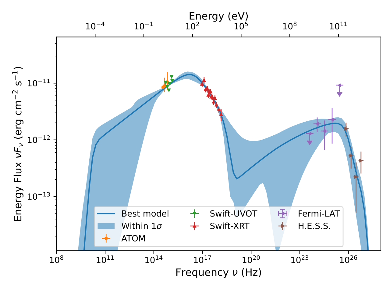
model_and_data.svg
Multiwavelength SED with data points, best model, and 1-sigma confidence level contours of the best model. Note the 1-sigma contours on this plot are an approximation of the real contours to save computation time. e.g.
particle_spectrum.svg
Particle spectrum with 1-sigma confidence level contours of the best model. e.g.

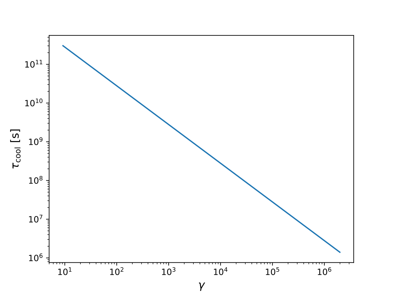
cooling_time_obs(Thomson).svg
Particle cooling time in the observer’s frame considering the Thomson regime.
\[\tau_\mathrm{cool}(\gamma) = \frac{3 m_e c}{4 (U_B + U'_\mathrm{rad}) \sigma_T \gamma} \frac{1+z}{\delta}\]With \(U_\mathrm{B}\) the magnetic field energy density and \(U'_\mathrm{rad}\) the sum of all soft photons radiation field densities in the blob’s frame. e.g.
.png)
\(\chi^2\) plots
\(\chi^2\) plots are critical to assess the convergence of the MCMC chain. They provide insights to the user in taking longer/shorter chains or changing the number of free parameters.
chi_squared_plot_all.jpeg
\(\chi^2\) of all individual walkers. e.g.

chi_squared_plot_best.svg
Best \(\chi^2\) at each step. e.g.

chi_squared_plot_med.svg
Median of all walker’s \(\chi^2\) at each step. Fitted with exponential decay function. e.g.

Corner plot
1D posterior probability distribution of each free parameter, 2D posterior probability distribution of each pair of parameters, best parameter, 1-sigma parameter range. e.g.
